SNV

Options

Option	Description	Argument
--samples	Sample names. It determines the plotting order. If “NA” all samples are used [default NA]	[char …]
--gipOut	GIP output directory [default gipOut]	[char]
--outName	Output name [default gipOut/sampleComparison/SNV]	[char]
--chrs	Chromosomes to use. If “NA” it uses the same chromsomes as GIP [default NA]	[char …]
--coordCartesianYlim	Max y-axis value for density plots If "NA" the value is automatically attributed [default NA]	[double]
--minVRF	Discard SNVs with frequency < –minVRF [default 0]	[double]
--maxVRF	Discard SNVs with frequency > –maxVRF [default 1]	[double]
--denLineSize	Density plot line thickness [default 1]	[double]
--SNVopacity	Opacity value of the dots representing SNVs. Max 1, Min 0 [default 1]	[double]
--showCoverage	Overlay sequencing coverage
--covLineSize	Coverage line thickness. DEPENDENCY –showCoverage [default 0.5]	[double]
--smoothingFactor	Merge and average the normalized coverage of this number of adjacent bins. DEPENDENCY –showCoverage [default 30]	[double]
--maxCov	Normalized coverage values > --maxCov are shown as --maxCov. DEPENDENCY –showCoverage [default 5]	[double]
--customColors	TSV file with 2 columns named “SAMPLE” and “COLOR” indicating the color to be used for each sample If “NA” colors are automatically assigned [default NA]	[char]
--randomSNVtoShow	Number of random SNV to show in scatterplots. If “NA” all SNVs are shown [default NA]	[integer]
--debug	Dump session and quit
-h, --help	Show help message

Description

The SNV module aims at comparing the SNV in terms of number, position and frequency for a samples set.

For each sample the module loads the GIP files with the filtered SNVs data (singleVariants.df.gz files) and generates multiple plots overlaying in different colors the SNVs sets.

Should a sample set present a huge number of SNVs (e.g. cancer samples) the user can specify the --randomSNVtoShow graphical options to set the maximum number of SNVs to be shown in scatterplots and reduce overplotting. This option does not affects the density profiles, which are in any case estimated using all selected SNVs, i.e. they are never based on a random SNV subset.

Example

From the GIP worked example folder execute

giptools SNV

This will generate the SNV output files in the gipOut/sampleComparison folder.

By default this module will consider all the GIP samples. Depending on the number of SNVs and the number of processed samples the resulting figures may be too dense and difficoult to read. The user can specify a sample subset with the --samples option.

In addition, this module offers the possibility to overlay the genomic bin sequencing coverage to the SNV frequency by specifying the --showCoverage option.

The giptools SNV --samples LIPA83 ZK28 ZK5 --showCoverage command produces the SNV.count.pdf reporting a stacked barplot with the number of SNVs for each chromosome and for each sample:

The SNV.overview.pdf and SNV.multipanel.pdf files offer an overview of all detected SNVs across the different chromosomes:

The SNV.density.pdf file provides a representation of the density distributions of the SNV frequencies in the different chromosomes:

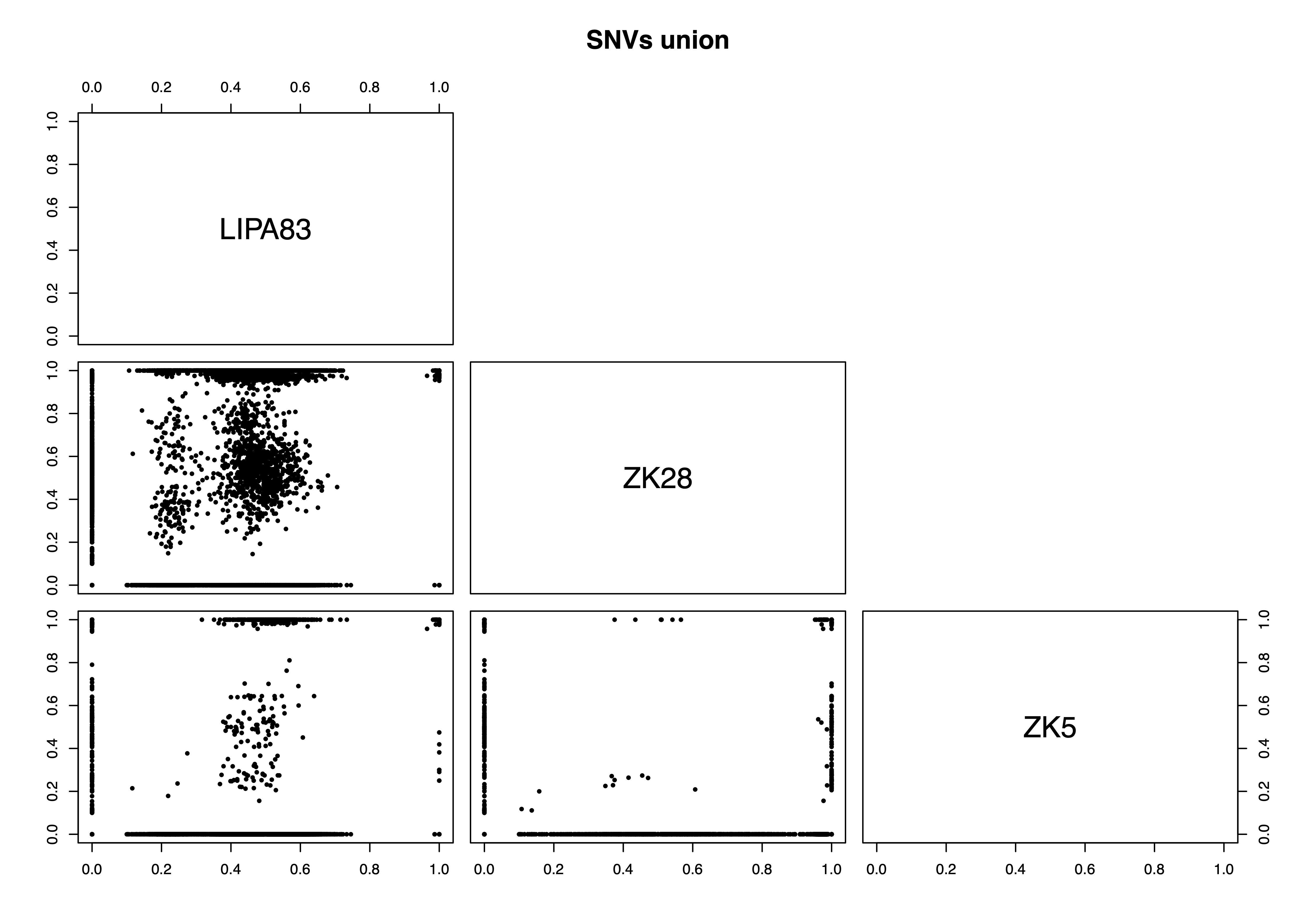
The SNV.pairwise.pdf files includes two plots demonstrating the frequency of detected SNVs in pairwise sample comparisons. The first plot represents the union of all SNVs detected across all samples processed with the giptools SNV module. The second plot show the intersection set, which includes just the SNVs detected (i.e. variant allele frequency > 0) in all the considered samples. The union plot fir this example is the following:

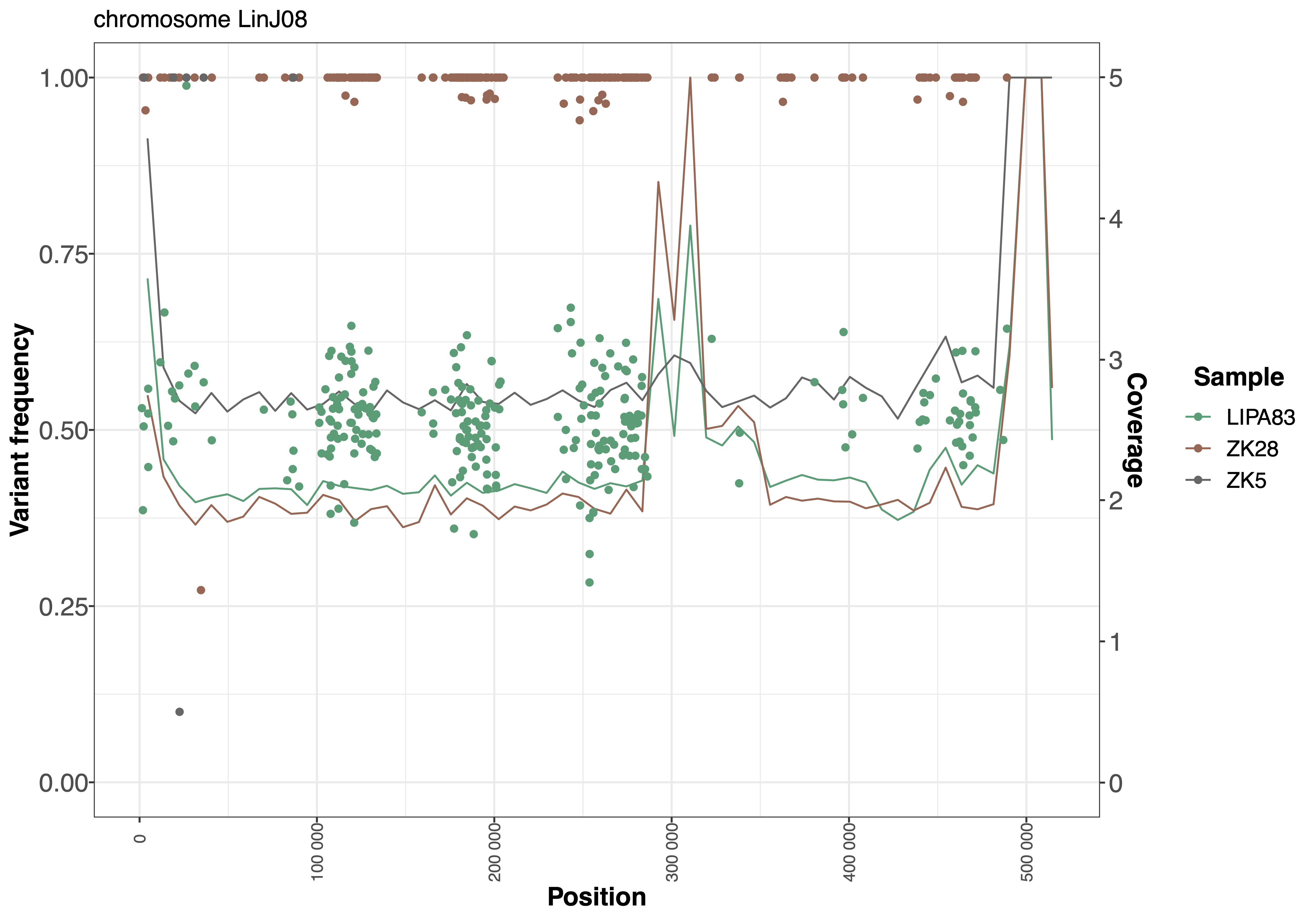
The SNV.byChr.pdf file includes one separate plot for each chromosome, showing the position and the variant allele frequency of detected SNVs. If the option --showCoverage is selected, these plots will include one line per sample showing the bin sequencing coverage. The plot produced for chromosome 8 in this example is the following:

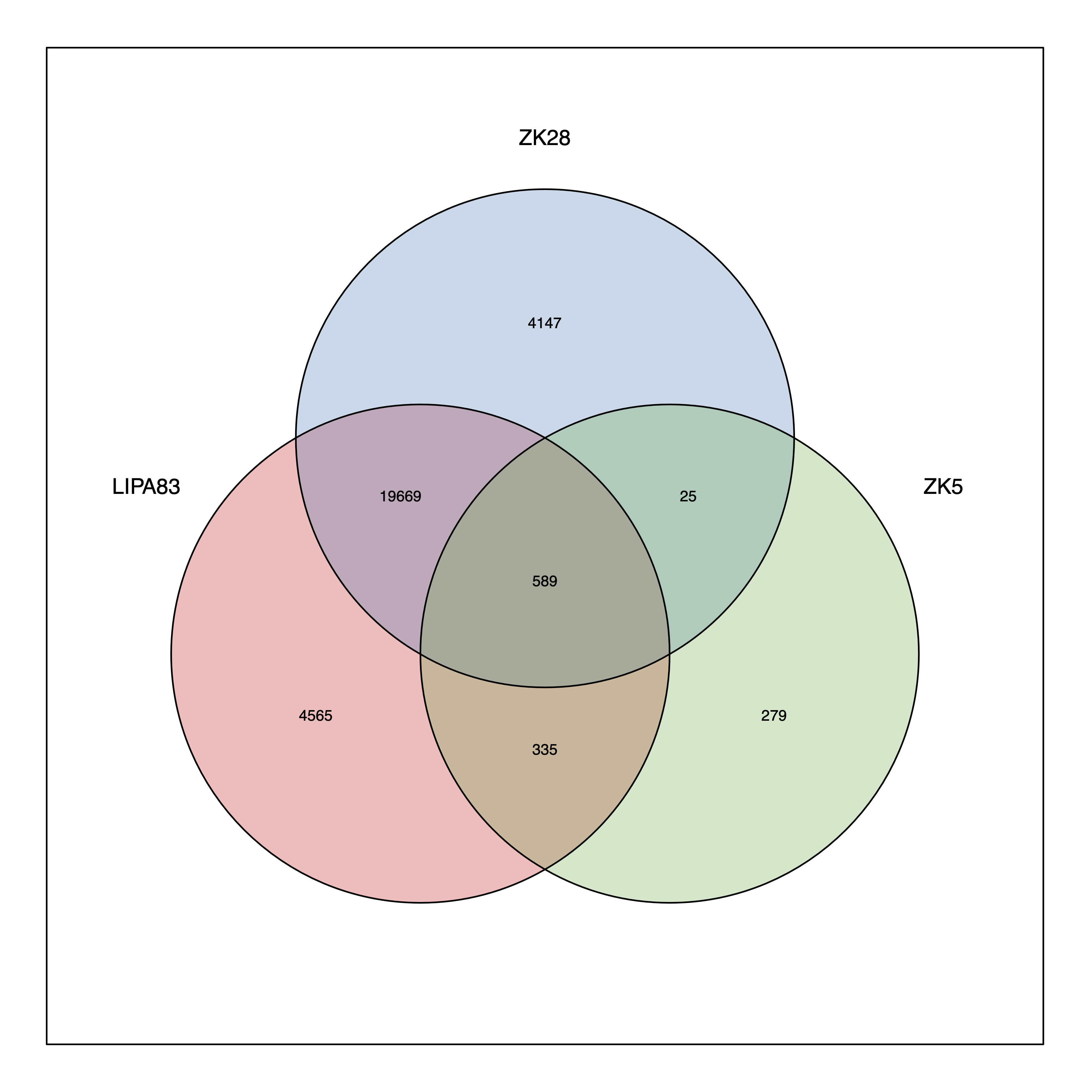
If the module analyzes less than 8 samples, then it will also generate the SNV.venn.pdf plot showing a Venn diagram demonstrating the number of unique and shared SNVs in the sample set:

The SNV.xlsx reports the list of SNVs with the variant allele frequency measured in each sample, and the predicted SNV effect.